
Real-time lane detection and tracking with a particle filter
General ·In this article, an algorithm for solving the lane tracking and detection using a Particle filter is proposed. The main objective was to reach a high accuracy in lane detection with a high velocity of execution so the algorithm can be implemented in a real-time system. It produces two splines that represent the lane markers. Detection and tracking of the lane were made in a particle filter in the same step thanks to the weighting function based directly on the colour of the pixels of the probability density matrix.
Introduction
It is common for self-driving devices to move in an environment that contains lane that the robots have to follow and so a lane detection and tracking algorithm is a key element for such systems. Lane detection refers to the analysis of an image to identify the lane. Lane tracking instead consists of introducing the history knowledge in the detection of the lane to obtain more accurate and faster results.
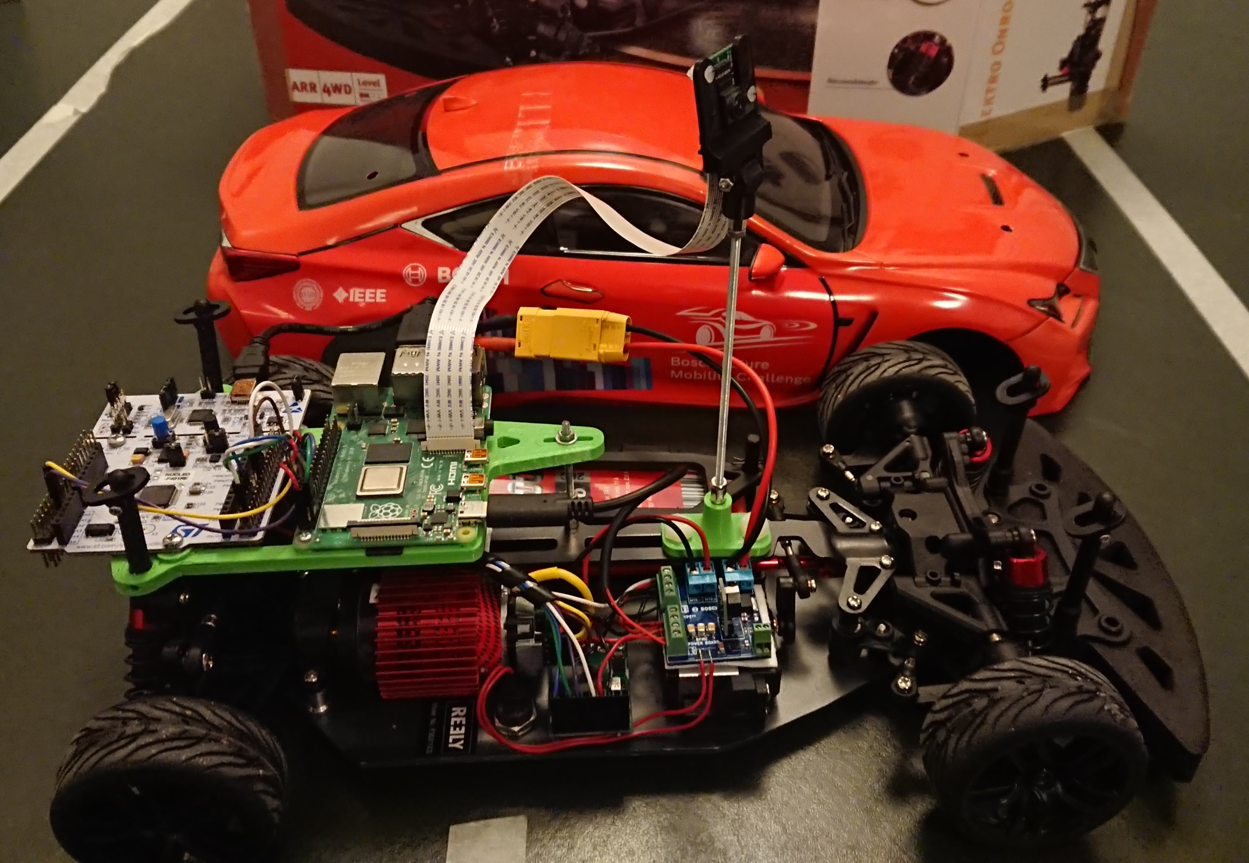
The objective of this project was to create a light algorithm that could do lane
detection and tracking in a Raspberry Pi using images obtained by a
PiCamera in real-time.
The method implemented consist of two main parts. The first part is the
image pre-processing that aim to create a Probability Density
Function(PDF) of lane markers starting from the pictures. The second module
is the particle filter using the output of the first module to do the
lane tracking and detection.
Related works
The most common approach for this kind of project is to develop three systems: lane feature extraction, lane detection and lane tracking.
Lane Feature extraction
This step is a fundamental one for the system since it extracts information from the pictures that will be used in the following steps, low quality in this phase will cause the failure of the algorithm.
The most common approaches used in this stage are edge-based techniques. They aim to recognize sharp discontinuity in images based on the intensity and contrast of the colour of the pixel in the pictures. There are multiple techniques to perform the edge detection like Canny, Sobel, Prewitt or Roberts that works with the maximums and minimums of the first derivative of the image for adjacent pixels and the Laplacian methods instead that works with the values that approach zero of the second derivative of the image.
A different system for Lane Feature extraction is the usage of Machine Learning that provides good result but it requires that the training set contains all the possible cases otherwise the system will not work in every situation.
Lane Detection
At this stage, the a priori knowledge of the road model is used to reduce the number of lines detected in the previous step. One of the most common techniques used is the Houg Transform. The high usage is due to the good result and the speed for lines detecting with the limit of the possibility to find only straight lines. The RANSAC method instead is very powerful for removing outliers and it works well with noises.
Another effective and simple method is based on a set of hypothesis created randomly. The hypotheses are lines that are candidate solution to represent the lane markers and they are weighted based on the likelihood that they are a real lane marker. The tracking stage will reduce the number of hypotheses needed and make this approach work.
Lane Tracking
At this step, the state of the vehicle is introduced in the algorithm to obtain more accurate estimations. The previous phases work only on one picture, now in this step, the data from the previous instants are used to approximate the lane with higher accuracy.
One of the most common approaches for Lane tracking is the Kalman Filter. The advantages of using this filter are the velocity and accuracy that it provides. The disadvantage is that the results are not accurate when data is noisy or when it runs on complex and unexpected situations as it is common for lane tracking as it could be crossroad, obstacles or bends. A better alternative is the Particle Filter. It uses a set of randomly generated particle that approximate the solution. The advantage is that it can describe complex states than the Kalman Filter.
However, Lane Tracking is not always used, it is also possible to detect the lane on a single picture without using information for the previous state of the vehicle.
Method
The system implemented takes as input images obtained from a camera sensor, one at a time, and produces as output two candidate lines that identify the street lane. The camera sensor is fixed on a forward locking position on top of a vehicle.
The input is processed to produce a PDF of the street lines. The initial colour image is transformed into a greyscale image where the intensity of a pixel indicates the probability that the pixel appertain to a street line. The particle filter used is the classic one. It starts with the initialization than sampling, weighting and resampling. The weighting is made using the PDF obtained in the initial step. All the steps are reported in the flowchart.
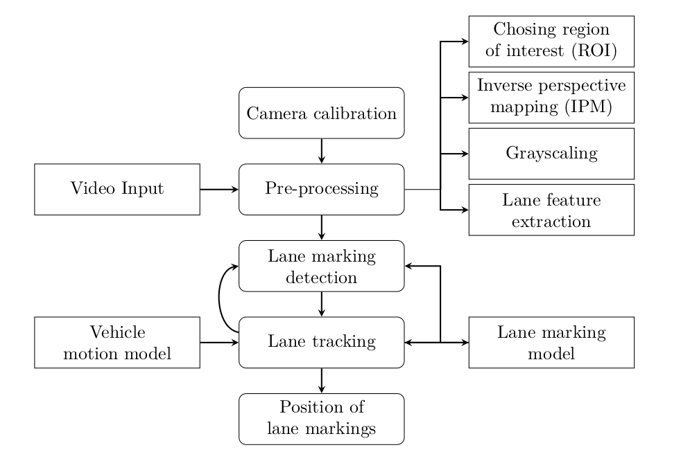
Image processing
To extract the best PDF, the input image is processed through multiple steps.
Initially, the image is cut so only the part of the image that contains the street is selected. The cut parameters are manually chosen before executing the algorithm. Choose the cutting points of the figure can be made without automation since the camera is fixed on the car and so the interesting part of the figure for controlling the car will be always fixed. The second cut operation is made to obtain two images, one that will contain the left line and one that will contain the right line.
Then an Inverse Perspective Mapping(IPM) is applied. In this way, the perspective effect due to the camera position in the car is decreased. The transformation is made using a 3x3 matrix that does a remapping of the picture.
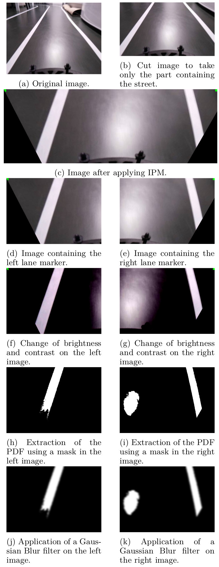
Then the brightness and the contrast of the images are edited to facilitate the extraction of the lines and reduce the light reflections parts of the image that can cause a wrong PDF. Finally, a filter is applied to extract only the part of the picture that contains white and yellow colours that are the possible colours of the lines in the dataset used.
The last step of the image processing is the application of a Gaussian Blur filter to remove some noisy and to transform the mask obtained in a probability density matrix that will permit the particle filter to converge better.
Particle filter
The objective is to identify the street lines and so a particle is a line and it is represented as a set of points as in the following equation.
\[\begin{aligned} \label{eq:line} p = \{(x_1, y_1), (x_2, y_2), ..., (x_{N_{c}}, y_{N_{c}})\} ~~~~ N_{c}\geq 2\end{aligned}\]where \((x_i,x_i), 0<i\leq N_{c}\) are the coordinates of the point that identify the line. If \(N_{c}=2\), then a particle is a straight line, instead, if \(N_{c}>2\) the points are interpolated using a spline or an open polygonal chain. Therefore a particle is also defined by the \(order\) of interpolation and the number of control points \(N_{c}\) and by changing them different particles can be obtained as shown in the following figure.
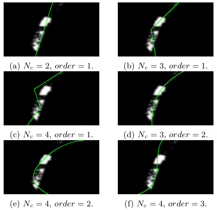
The number of particles used in the filter will be denoted with \(N_{p}\). The algorithm is implemented in a way that both straight lines and splines can be used. Using the particle filter on the straight lines permit to obtain a faster execution because is less computationally expensive to do the calculations but the spline has the advantage of approximating better curves instead of straight lines.
Two particle filter are used in the algorithm, one work on the left part of the image trying to approximate the left lane marker, one the right marker. The final output of the algorithm is two lines that identify a lane.
Particle initialization
This first step of the algorithm creates the initial set of particles by generating the points that describe each particle. The ordinate of the points is fixed so the points are uniformly spread for all the heigh of the image. This choice comes from the model of the road and so from the fact that lane markers will go across the whole picture from top to bottom. The abscissa is selected randomly using a Gaussian distribution.
\[\begin{aligned} \label{eq:y} y_i = (i-1) * image\_heigh/(N_{c} - 1) ~~~~ 0\leq i \leq N_{c}\end{aligned}\]At the end of this step, the weight of each particle is set to \(1/N_{p}\).
Line sampling
In this step, the particle filter creates new particles by changing the x-coordinate of all the points of the particles. It does not act on the y-coordinate since it is always expected to have two lines that cross all the input image vertically. The x-coordinate is updated using a new value evaluated from a Gaussian distribution as expressed in the equation:
\[\begin{aligned} \label{eq:x_sampling} x^{(new)}_i = \mathcal{N}(x_i, \sigma_i) ~~~~ 0<i<=N_{c}\end{aligned}\]When the car turns, the points on the image that corresponds to the points more father from the car will move faster. To take that in consideration, \(\sigma\) is evaluated using the equation:
\[\begin{aligned} \label{eq:sigma} \sigma_i=((N_{c}-1) - i) * 40/N_{c} + 5\end{aligned}\]Line weightings
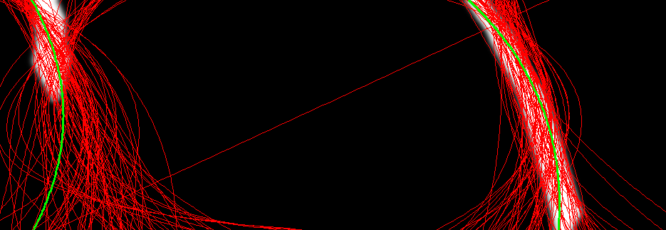
This step is central to have a particle filter that converges to the right line. The approach used is computationally simple. The weight of a line is equal to the sum of the pixel colour of the line projection on the PDF as shown in the following figure.
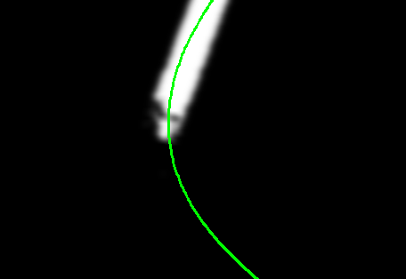
As a result of the previous image processing, the PDF is composed of pixels that have a value in the range \([0,1]\).
A particle is weighted by passing through two steps. Firstly \(M\) points are created by interpolating the particle control points as expressed in equation:
\[\begin{aligned} \label{eq:weight_interpolate} Q=\{q_0, q_1, ...,q_M\}=interpolate(p, M)\end{aligned}\]Secondly, weights are evaluated by summing the value of the PDF at the coordinates of the points of \(Q\). The iteration over \(p\) and \(q\) are used for giving a thickness to the lines and help the algorithm to converge.
\[\begin{aligned} \label{eq:weight} W_i=\sum\limits_{i=0}^M \sum\limits_{j=-1}^1 \sum\limits_{k=-1}^1 pdf(q_{i,x}+j, q_{i,y}+k)\end{aligned}\]Line resampling
The resampling was made using Systematic resampling. This approach consists of choosing an initial random number and then select the particle using a fixed distance. It was chosen because is fast since only one random number is needed and because it guarantees a better variance than totally random sampling and so it reduces the possibility of too fast convergence.
Line extraction
From the set of particles, two methods were implemented to extract the final line to use as an approximation of the real line. The first method consists to simply select the particle with the highest weight and so the one that overlaps more the street lane marker. The second method instead consists in creating a new particle where the x-coordinates of the points are the averages of the x-coordinates of all the points of the particle set as expressed in the equation:
\[\label{eq:avgApproximation} \begin{aligned} p_{approx} = \{(avg(p_{i_{x_1}}), y_1), (avg(p_{i_{x_2}}), y_2), \\..., (avg(p_{i_{x_{N_c}}}), y_{N_{c}})\} \\ 0<=i<=N_{p} \end{aligned}\]where \(avg\) makes the average of a list of number, \(N_{p}\) is the number of particles and \(p_{i_{x_j}}\) indicates the \(x\) coordinate of the \(j-\)th point of the \(i\)-th particle. The average method works only if the algorithm is converging in a region otherwise it creates a wrong line.
Reset mechanism
The particle filter implementation was extended including a module to reset the set of particles. If the particle that approximates the whole set has a weight lower than a certain threshold, \(20\%\) of the maximum weight, it means that the algorithm diverged. When the algorithm is not able to converge back to a good state after multiple instants, the set of particles is initialized from scratch using the initialization function. That’s important when the lane markers are lost due to fast change of direction, obstacles or other unexpected situation of the street.
Implementation
The programming language used to implement the system is Python 3. All the image processing operations were made using OpenCV 4.4.0 because it is very powerful and it permits to have access to a wide range of operations on images simplifying the creation of the system. The library Numpy was used to manage the operation on the PDF matrices. For interpolating the points presented in the particle the library Scipy was used.
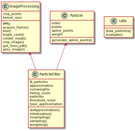
The code was structured using the object programming approach. This framework was used to simplify the debug, the readability of the code and the analysis of the system implemented. The negative point of this implementation is that it needs some extra loop that could be avoided using matrices representation and by removing some objects.
Result
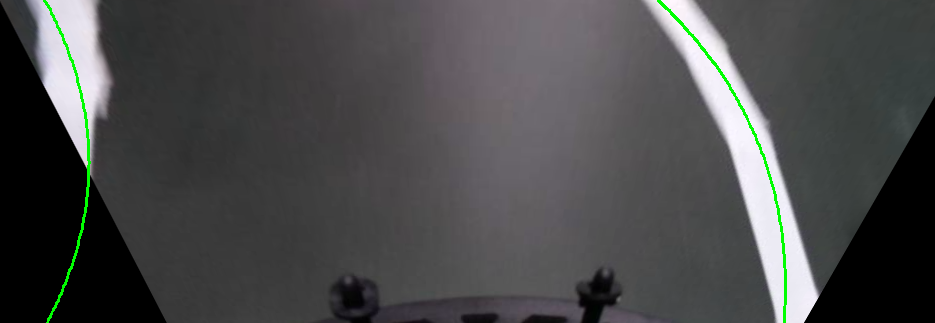
The algorithm was executed using video recorded in a close environment. The result can be seen in the following video.
From the video is possible to see that the Particle Filter perform well when the probability density function in input doesn’t have noise. Instead when the input image present reflections or complex light condition, the image processing algorithm fails to create a correct probability density function and so the lane detection fails.
In the report of this project, the influence of the main parameters in the algorithm is analyzed and a more detailed analysis of the result is discussed.
Conclusion
In this article, an algorithm for lane detection and tracking is proposed using a particle filter. The algorithm works and can find and track the lane markers in a simple environment. In the real world, the algorithm would probably have problems to create a correct PDF due to the complex light conditions and colours of the pictures. Even with some limitations, the algorithm can provide an estimation of the lane in real-time.
Future improvements
The project could be improved in different aspects. The sampling stage of the particle filter could be changed by including odometry information from the vehicle. In particular, the information about the turning of the steering wheel could be used to sample with less randomicity. A simple model, for example, could be to sample more lines in the direction of the turning of the steering wheel.
Another improvement regards the implementation of the algorithm. The code was implemented by balancing velocity of the execution and capacity of editing and debugging but it can be improved by removing some object and using matrices to represent the particles and so creating a faster algorithm. Moreover, other languages faster than Python, as C could be used and a GPU for image processing.
Another direction that should be taken would be on the image pre-processing. In this paper, the blur, brightness, contrast and a fixed mask were used to extract the PDF from the images but the three parameters were chosen at the beginning of the execution. That’s an optimal solution if the environment is without noise and in perfect light conditions. A better pre-processing of the image would not be fixed but the parameters would adapt to the pictures.
This article refers to the code present in this github repository. Detailed information on the code and on how to run the algorithm is in the README.md of the repository. A more complete analysis of the algorithm, of the results and the references of the background studies, can be found in the report of the project.
For any clarification and question feel free to contact me using the contact form, opening a new issue in the repository of the project or by leaving a comment under this post.